翻译|Gradient Descent in Python

翻译|Gradient Descent in Python

1
2
3
import numpy as np
import matplotlib.pyplot as plt
%matplotlib inline
1
plt.style.use(['ggplot'])

当你初次涉足机器学习时,你学习的第一个基本算法就是 梯度下降 (Gradient Descent), 可以说梯度下降法是机器学习算法的支柱。 在这篇文章中,我尝试使用 `python` 解释梯度下降法的基本原理。一旦掌握了梯度下降法,很多问题就会变得容易理解,并且利于理解不同的算法。

如果你想尝试自己实现梯度下降法, 你需要加载基本的 \(python\) \(packages\) —— \(numpy\) and \(matplotlib\)

首先, 我们将创建包含着噪声的线性数据

1
2
3
# 随机创建一些噪声
X = 2 * np.random.rand(100, 1)
y = 4 + 3 * X + np.random.randn(100, 1)

接下来通过 matplotlib 可视化数据

1
2
3
4
5
# 可视化数据
plt.plot(X, y, 'b.')
plt.xlabel("$x$", fontsize=18)
plt.ylabel("$y$", rotation=0, fontsize=18)
plt.axis([0, 2, 0, 15])

显然, `y` 与 `x` 具有良好的线性关系,这个数据非常简单,只有一个自变量 `x`.

我们可以将其表示为简单的线性关系:

$$
y = b + mx
$$

并求出 `b` , `m`。

这种被称为解方程的分析方法并没有什么不妥,但机器学习是涉及矩阵计算的,因此我们使用矩阵法(向量法)进行分析。

我们将 `y` 替换成 \(J(\theta)\), `b` 替换成 \(\theta_0\), `m` 替换成 \(\theta_1\)。
得到如下表达式:

$$
J(\theta) = \theta_0 + \theta_1 x
$$

注意: 本例中 \(\theta_0 = 4\), \(\theta_1 = 3\)

求解 \(\theta_0\) 和 \(\theta_1\) 的分析方法,代码如下:

1
2
3
X_b = np.c_[np.ones((100, 1)), X] # 为X添加了一个偏置单位,对于X中的每个向量都是1
theta_best = np.linalg.inv(X_b.T.dot(X_b)).dot(X_b.T).dot(y)
theta_best
array([[3.86687149],
       [3.12408839]])

不难发现这个值接近真实的 \(\theta_0\),\(\theta_1\),由于我在数据中引入了噪声,所以存在误差。

1
2
3
4
X_new = np.array([[0], [2]])
X_new_b = np.c_[np.ones((2, 1)), X_new]
y_predict = X_new_b.dot(theta_best)
y_predict
array([[ 3.86687149],
       [10.11504826]])

梯度下降法 (Gradient Descent)

Cost Function & Gradients

计算代价函数和梯度的公式如下所示。

注意:代价函数用于线性回归,对于其他算法,代价函数是不同的,梯度必须从代价函数中推导出来。

Cost

$$
\begin{equation}
J(\theta) = 1/2m \sum_{i=1}^{m} (h(\theta)^{(i)} - y^{(i)})^2
\end{equation}
$$

Gradient

$$
\begin{equation}
\frac{\partial J(\theta)}{\partial \theta_j} = 1/m\sum_{i=1}^{m}(h(\theta^{(i)} - y^{(i)}).X_j^{(i)}
\end{equation}
$$

Gradients

\begin{equation}
\theta_0: = \theta_0 -\alpha . (1/m .\sum_{i=1}^{m}(h(\theta^{(i)} - y^{(i)}).X_0^{(i)})
\end{equation}

\begin{equation}
\theta_1: = \theta_1 -\alpha . (1/m .\sum_{i=1}^{m}(h(\theta^{(i)} - y^{(i)}).X_1^{(i)})
\end{equation}

\begin{equation}
\theta_2: = \theta_2 -\alpha . (1/m .\sum_{i=1}^{m}(h(\theta^{(i)} - y^{(i)}).X_2^{(i)})
\end{equation}

\begin{equation}
\theta_j: = \theta_j -\alpha . (1/m .\sum_{i=1}^{m}(h(\theta^{(i)} - y^{(i)}).X_0^{(i)})
\end{equation}

1
2
3
4
5
6
7
8
9
10
11
12
13
14
15
16
17
def cal_cost(theta, X, y):
'''
Calculates the cost for given X and Y. The following shows and example of a single dimensional X
theta = Vector of thetas
X = Row of X's np.zeros((2,j))
y = Actual y's np.zeros((2,1))

where:
j is the no of features
'''

m = len(y)

predictions = X.dot(theta)
cost = (1/2*m) * np.sum(np.square(predictions - y))

return cost
1
2
3
4
5
6
7
8
9
10
11
12
13
14
15
16
17
18
19
20
21
22
23
24
25
def gradient_descent(X, y, theta, learning_rate = 0.01, iterations = 100):
'''
X = Matrix of X with added bias units
y = Vector of Y
theta=Vector of thetas np.random.randn(j,1)
learning_rate
iterations = no of iterations

Returns the final theta vector and array of cost history over no of iterations
'''

m = len(y)
# learning_rate = 0.01
# iterations = 100

cost_history = np.zeros(iterations)
theta_history = np.zeros((iterations, 2))
for i in range(iterations):
prediction = np.dot(X, theta)

theta = theta - (1/m) * learning_rate * (X.T.dot((prediction - y)))
theta_history[i, :] = theta.T
cost_history[i] = cal_cost(theta, X, y)

return theta, cost_history, theta_history
1
2
3
4
5
6
7
8
9
# 从1000次迭代开始,学习率为0.01。从高斯分布的θ开始
lr =0.01
n_iter = 1000
theta = np.random.randn(2, 1)
X_b = np.c_[np.ones((len(X), 1)), X]
theta, cost_history, theta_history = gradient_descent(X_b, y, theta, lr, n_iter)

print('Theta0: {:0.3f},\nTheta1: {:0.3f}'.format(theta[0][0],theta[1][0]))
print('Final cost/MSE: {:0.3f}'.format(cost_history[-1]))
Theta0:          3.867,
Theta1:          3.124
Final cost/MSE:  5457.747
1
2
3
4
5
6
# 绘制迭代的成本图
fig, ax = plt.subplots(figsize=(12,8))

ax.set_ylabel('J(Theta)')
ax.set_xlabel('Iterations')
ax.plot(range(1000), cost_history, 'b.')

在大约 150 次迭代之后代价函数趋于稳定,因此放大到迭代200,看看曲线

1
2
fig, ax = plt.subplots(figsize=(10,8))
ax.plot(range(200), cost_history[:200], 'b.')

值得注意的是,最初成本下降得更快,然后成本降低的收益就不那么多了。 我们可以尝试使用不同的学习速率和迭代组合,并得到不同学习率和迭代的效果会如何。

让我们建立一个函数,它可以显示效果,也可以显示梯度下降实际上是如何工作的。

1
2
3
4
5
6
7
8
9
10
11
12
13
14
15
16
17
18
19
20
21
22
23
24
25
26
27
def plot_GD(n_iter, lr, ax, ax1=None):
'''
n_iter = no of iterations
lr = Learning Rate
ax = Axis to plot the Gradient Descent
ax1 = Axis to plot cost_history vs Iterations plot
'''

ax.plot(X, y, 'b.')
theta = np.random.randn(2, 1)

tr = 0.1
cost_history = np.zeros(n_iter)
for i in range(n_iter):
pred_prev = X_b.dot(theta)
theta, h, _ = gradient_descent(X_b, y, theta, lr, 1)
pred = X_b.dot(theta)

cost_history[i] = h[0]

if ((i % 25 == 0)):
ax.plot(X, pred, 'r-', alpha=tr)
if tr < 0.8:
tr += 0.2

if not ax1 == None:
ax1.plot(range(n_iter), cost_history, 'b.')
1
2
3
4
5
6
7
8
9
10
11
12
13
14
15
16
17
# 绘制不同迭代和学习率组合的图
fig = plt.figure(figsize=(30,25), dpi=200)
fig.subplots_adjust(hspace=0.4, wspace=0.4)

it_lr = [(2000, 0.001), (500, 0.01), (200, 0.05), (100, 0.1)]
count = 0
for n_iter, lr in it_lr:
count += 1

ax = fig.add_subplot(4, 2, count)
count += 1

ax1 = fig.add_subplot(4, 2, count)

ax.set_title("lr:{}" .format(lr))
ax1.set_title("Iterations:{}" .format(n_iter))
plot_GD(n_iter, lr, ax, ax1)

通过观察发现,以较小的学习速率收集解决方案需要很长时间,而学习速度越大,学习速度越快。

1
2
_, ax = plt.subplots(figsize=(14, 10))
plot_GD(100, 0.1, ax)

随机梯度下降法(Stochastic Gradient Descent)

随机梯度下降法,其实和批量梯度下降法原理类似,区别在与求梯度时没有用所有的 `m` 个样本的数据,而是仅仅选取一个样本 `j` 来求梯度。对应的更新公式是:

$$
\theta_i = \theta_i - \alpha (h_\theta(x_0^{(j)}, x_1^{(j)}, …x_n^{(j)}) - y_j)x_i^{(j)}
$$

1
2
3
4
5
6
7
8
9
10
11
12
13
14
15
16
17
18
19
20
21
22
23
24
25
26
27
def stocashtic_gradient_descent(X, y, theta, learning_rate=0.01, iterations=10):
'''
X = Matrix of X with added bias units
y = Vector of Y
theta=Vector of thetas np.random.randn(j,1)
learning_rate
iterations = no of iterations

Returns the final theta vector and array of cost history over no of iterations
'''

m = len(y)
cost_history = np.zeros(iterations)

for it in range(iterations):
cost = 0.0
for i in range(m):
rand_ind = np.random.randint(0, m)
X_i = X[rand_ind, :].reshape(1, X.shape[1])
y_i = y[rand_ind, :].reshape(1, 1)
prediction = np.dot(X_i, theta)

theta -= (1/m) * learning_rate * (X_i.T.dot((prediction - y_i)))
cost += cal_cost(theta, X_i, y_i)
cost_history[it] = cost

return theta, cost_history
1
2
3
4
5
6
7
8
lr = 0.5
n_iter = 50
theta = np.random.randn(2,1)
X_b = np.c_[np.ones((len(X),1)), X]
theta, cost_history = stocashtic_gradient_descent(X_b, y, theta, lr, n_iter)

print('Theta0: {:0.3f},\nTheta1: {:0.3f}' .format(theta[0][0],theta[1][0]))
print('Final cost/MSE: {:0.3f}' .format(cost_history[-1]))
Theta0:          3.762,
Theta1:          3.159
Final cost/MSE:  46.964
1
2
3
4
5
6
7
fig, ax = plt.subplots(figsize=(10,8))

ax.set_ylabel('$J(\Theta)$' ,rotation=0)
ax.set_xlabel('$Iterations$')
theta = np.random.randn(2,1)

ax.plot(range(n_iter), cost_history, 'b.')

小批量梯度下降法(Mini-batch Gradient Descent)

小批量梯度下降法是批量梯度下降法和随机梯度下降法的折衷,也就是对于 `m` 个样本,我们采用 `x` 个样子来迭代,\(1<x<m\)。一般可以取 `x=10`,当然根据样本的数据,可以调整这个 `x` 的值。对应的更新公式是:

$$
\theta_i = \theta_i - \alpha \sum\limits_{j=t}^{t+x-1}(h_\theta(x_0^{(j)}, x_1^{(j)}, …x_n^{(j)}) - y_j)x_i^{(j)}
$$

1
2
3
4
5
6
7
8
9
10
11
12
13
14
15
16
17
18
19
20
21
22
23
24
25
26
27
28
29
30
31
32
def minibatch_gradient_descent(X, y, theta, learning_rate=0.01, iterations=10, batch_size=20):
'''
X = Matrix of X without added bias units
y = Vector of Y
theta=Vector of thetas np.random.randn(j,1)
learning_rate
iterations = no of iterations

Returns the final theta vector and array of cost history over no of iterations
'''

m = len(y)
cost_history = np.zeros(iterations)
n_batches = int(m / batch_size)

for it in range(iterations):
cost = 0.0
indices = np.random.permutation(m)
X = X[indices]
y = y[indices]
for i in range(0, m, batch_size):
X_i = X[i: i+batch_size]
y_i = y[i: i+batch_size]

X_i = np.c_[np.ones(len(X_i)), X_i]
prediction = np.dot(X_i, theta)

theta -= (1/m) * learning_rate * (X_i.T.dot((prediction - y_i)))
cost += cal_cost(theta, X_i, y_i)
cost_history[it] = cost

return theta, cost_history
1
2
3
4
5
6
7
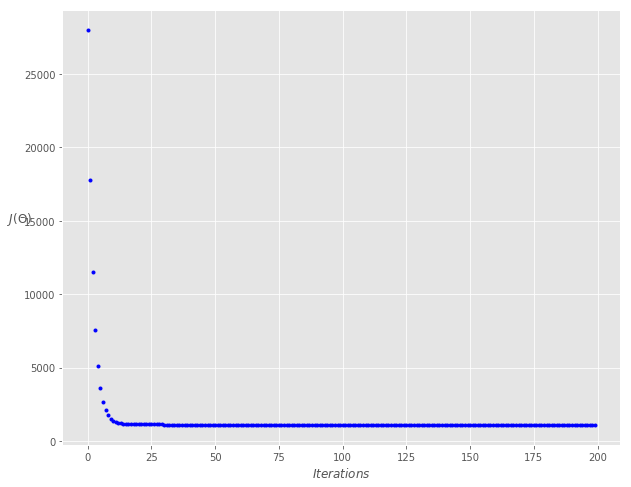
lr = 0.1
n_iter = 200
theta = np.random.randn(2, 1)
theta, cost_history = minibatch_gradient_descent(X, y, theta, lr, n_iter)

print('Theta0: {:0.3f},\nTheta1: {:0.3f}' .format(theta[0][0], theta[1][0]))
print('Final cost/MSE: {:0.3f}' .format(cost_history[-1]))
Theta0:          3.842,
Theta1:          3.146
Final cost/MSE:  1090.518
1
2
3
4
5
6
7
fig, ax = plt.subplots(figsize=(10,8))

ax.set_ylabel('$J(\Theta)$', rotation=0)
ax.set_xlabel('$Iterations$')
theta = np.random.randn(2, 1)

ax.plot(range(n_iter), cost_history, 'b.')

参考

评论

Your browser is out-of-date!

Update your browser to view this website correctly. Update my browser now

×